Modeling field goal kicking – part III

Now that we have formed our prior beliefs, we’ll summarize the posterior by computing the density on a fine grid of points.  The functions mycontour and simcontour in the LearnBayes package are helpful here.

After loading LearnBayes, the logarithm of the  logistic posterior is programmed in the function logisticpost.  There are two arguments to this posterior, the vector theta of regression coefficients and the data which is a matrix of the form [s n x], where s is the vector of successes, n is the vector of sample sizes, and x is the vector of covariates.  When we use the conditional means prior (described in the previous post), the prior is in that form, so we simply augment the data with the prior “data” and that is the input for logisticpost.

Here is the matrix prior that uses the parameters described in the previous post.

prior=rbind(c(30, 8.25 + 1.19, 8.25),
            c(50, 4.95 + 4.95, 4.95))

We paste the data and prior together in the matrix data.prior.

data.prior=rbind(d, prior)

After some trial and error, we find that the rectangle
(-2, 12, -0.3, 0.05) brackets the posterior.  We draw a contour plot of the posterior using the mycontour function — the arguments are the function defining the log posterior, the vector of limits (xlo, xhi, ylo, yhi) and the data.prior matrix.

mycontour(logisticpost, c(-2, 12, -0.3, 0.05), data.prior,
    xlab=expression(beta[0]), ylab=expression(beta[1]))

Now that we have bracketed the posterior, we use the simcontour function to take a simulated sample from the posterior.

S=simcontour(logisticpost, c(-2, 12, -.3, .05), data.prior, 1000)

I place the points on the contour to demonstrate that this seems to be a reasonable sample.

points(S)

Let’s illustrate doing some inference.  Suppose I’m interested in p(40), the probability of success at 40 yards.  This is easy to do using the simulated sample.  I compute values of p(40) from values of the simulated draws of and then construct a density estimate of the simulated draws.

p40 = exp(S$x + 40*S$y)/(1 + exp(S$x + 40*S$y))
plot(density(p40))

I’m pretty confident that the success rate from this distance is between 0.6 and 0.8.

 

Modeling Field Goal Kicking — part 2

Let’s continue the football kicking example.

1.  Prior beliefs.  On the surface, it seems challenging to talk about prior information since the regression parameters and are not very meaningful.  But we might have some beliefs about the probability of kicking a goal successful and we can use these beliefs to indirectly construct a prior on the regression coefficients.

2.  Conditional means prior.  We instead consider the parameters (p(30) and p(50)), the probabilities of successfully kicking a field goal at 30 yards and 50 yards.  After some thought, I believe:

• The median and 90th percentile at p(30) are respectively 0.90 and 0.98  (I’m pretty confident of a successful kick at 30 yards.)
• The median and 90th percentile at p(50) are respectively 0.50 and 0.70. (I’m less confident of a successful kick of 50 yards.)

Assuming my beliefs about p(30) and p(50) are independent, and assuming beta priors, my joint prior is given by

where are the matching beta shape parameters found using a function like beta.select in the LearnBayes package.

3.  Then we can transform this prior on (p(30), p(50)) to a density on .  It can be shown that this transformed prior has a product of betas form which makes it very convenient to use.

The log of the logistic likelihood is actually a function logisticpost in the LearnBayes package, and it is convenient to use it for this example.

Modeling Field Goal Kicking

Since it is (American) football season, it seemed appropriate to do a football example to illustrate summarizing a bivariate posterior.

One way of scoring points in football is by kicking field goals.  The ball is lined up at a particular location on the field and the kicker attempts to kick the ball through the uprights.

We are interested in looking at the relationship between the distance of the attempt (in yards) and the result of the kick (success and failure).  I collect the results of 31 field goal attempts for the Big Ten college games in the second week of the 2011 season.   I read the data into R from the class web folder and display the beginning of the data frame fieldgoal:

> fieldgoal=read.csv("http://personal.bgsu.edu/~albert/MATH6480/DATA/fieldgoal.csv")
> head(fieldgoal)
  Distance Result
1       42      1
2       54      1
3       20      1
4       42      0
5       50      1
6       38      0

A logistic model can be used to represent this data.  Let denote the result of the th kick at distance — either the kick is good () or it is missed ().  Let denote the probability that .  A simple logistic model says that

The standard way of fitting this model is based on maximum likelihood based on the iterative reweighted least-squares algorithm.  We can implement this algorithm using the R glm function with the family = binomial argument.

> glm(Result ~ Distance, family = binomial, data = fieldgoal)

Coefficients:
(Intercept)     Distance
    3.81329     -0.07549

As expected, the slope is negative — this means that it is harder to make a field goal for a longer distance.

We’ll use this example in a future post to illustrate prior modeling and “brute force” computation of the posterior.

Bayesian regression – part II

In the earlier posting (part I), I demonstrated how one obtains a prior using a portion of the data and then uses this as a prior with the remaining portion of the data to obtain the posterior.

One advantage of using proper priors is that one can implement model selection.

Recall that the output of the MCMCregress function was fit2 — this is the regression model including all four predictors Food, Decor, Service, and East.

Suppose I want to compare this model with the model that removes the Food variable.  I just adjust my prior.  If I don’t believe this variable should be in the model, my prior for that regression coefficient should be 0 with a tiny variance or a large precision.   Currently my prior mean is stored in the variable beta0 and the precision matrix is stored in B0.   I change the component of beta0 corresponding to Food to be 0 and then assign a really big value to the (Food, Food) entry in the precision matrix B0.  I rerun MCMCregress using this new model and the output is stored in fit2.a.

beta0.a=beta0; beta0.a[2]=0
B0.a=B0; B0.a[2,2]=200000
fit2.a=MCMCregress(Price~Food+Decor+Service+East,
data = italian2, burnin = 0, mcmc = 10000,
thin = 1, verbose = 0, seed = NA, beta.start = NA,
b0 = beta0.a, B0 = B0.a, c0 = c0, d0 = d0,
marginal.likelihood = c(“Chib95”))

To compare the two models (the full one and the one with Food removed), I use the BayesFactor function in MCMCpack.  This gives the log marginal likelihood for each model and compares models by Bayes factors.  Here is the key output.

BayesFactor(fit2,fit2.a)
The matrix of the natural log Bayes Factors is:

fit2 fit2.a
fit2      0    303
fit2.a -303      0

On the ln scale, the full model is far superior to the model with Food removed since the log Bayes factor in support of the full model is 303.  Clearly, Food must be an important variable.

By the way, in LearnBayes, I have a function bayes.model.selection that implements Bayesian model selection using a g-prior on the regression coefficients.   This function gives reasonable results for this example.

Logistic regression exercise

In my Bayesian class, I assigned a problem (exercise 8.3 from BCWR) where one is using logistic regression to model the trajectory of Mike Schmidt’s home run rates.

First, I have written a function to compute the log posterior for a logistic regression model with a vague prior placed on the regression vector.  The function together with a short example how it works can be found here.

Second, it seems that there is a problem getting the laplace function to converge if you don’t use a really good starting value.  Here is an alternative way of getting the posterior mode.

Suppose y is a vector containing the home run counts and n is a vector with the sample sizes.  Let age be the vector of ages and age2 be the vector of ages squared.  Define the response to be a matrix containing the vectors of successes and failures.

response=cbind(y,n-y)

Then the mle of beta is found using the glm command with the family=binomial option

fit=glm(response~age+age2,family=binomial)

The posterior mode is the mle:

beta=coef(fit)

The approximation to the posterior variance-covariance matrix is found by

V=vcov(fit)

Now you should be able to use the random walk metropolis algorithm to simulate from the posterior.

Bayesian regression — part I

To illustrate Bayesian regression, I’ll use an example from Simon Sheather’s new book on linear regression.  A restaurant guide collects a number of variables from a group of Italian restaurants in New York City.  One is interested in predicting the Price of a meal based on Food (measure of quality), Decor (measure of decor of the restaurant), Service (measure of quality of service), and East (dummy variable indicating if the restaurant is east or west of 5th Avenue).

Here is the dataset in csv format:  http://www.stat.tamu.edu/~sheather/book/docs/datasets/nyc.csv

Assuming the usual regression model

, ,

suppose we assign the following prior to :  we assume independence with and .  Here is the precision matrix, the inverse of the variance-covariance matrix.

How do we obtain values of the parameters ?  We’ll use a small part of the data to construct our prior, and then use the remaining part of the data to do inference and eventually do some model selection.

First, I read in the data, select a random sample of rows, and partition the data into the two datasets italian1 and italian2.

italian=read.csv(“http://www.stat.tamu.edu/~sheather/book/docs/datasets/nyc.csv”)
indices=sample(168,size=25)
italian1=italian[indices,]
italian2=italian[-indices,]

I use the function blinreg in the LearnBayes package to simulate from the posterior using a vague prior.

library(LearnBayes)
y=italian1$Price
X=with(italian1,cbind(1,Food,Decor,Service,East))
fit=blinreg(y,X,5000)

From the simulated draws, I can now get estimates of my prior.  The parameters for the normal prior on are found by finding the sample mean and sample var-cov matrix of the simulated draws.  The precision matrix is the inverse of the var-cov matrix.  The parameters correspond to the sum of squared errors and degrees of freedom of my initial fit.

beta0=apply(fit$beta,2,mean)
Sigma0=cov(fit$beta)
B0=solve(Sigma0)
c0=(25-5)
d0=sum((y-X%*%beta0)^2)

The function MCMCregress in the MCMCpack package will simulate from the posterior of using this informative prior.  It seems pretty to use.  I show the function including all of the arguments.  Note that  I’m using the second part of the data italian2, I input my prior through the b0, B0, c0, d0 arguments, and I’m going to simulate 10,000 draws (through the mcmc=10000 input).

fit2=MCMCregress(Price~Food+Decor+Service+East,
data = italian2, burnin = 0, mcmc = 10000,
thin = 1, verbose = 0, seed = NA, beta.start = NA,
b0 = beta0, B0 = B0, c0 = c0, d0 = d0,
marginal.likelihood = c(“Chib95”))

The output of MCMCregress, fit2, is a MCMC object that one can easily summarize and display using the summary and plot methods in the coda package.

Suppose we are interested in estimating the mean price at a restaurant on the east side (east = 1) with Food = 30, Decor = 30 and Service = 30.  We define a row matrix that consists of these covariates.  Then we compute the linear predictor for each of the simulated beta vectors.  The vector lp contains 10,000 draws from the posterior of .

x=matrix(c(1,20,20,20,1),5,1)
beta=fit2[,1:5]
sigma=sqrt(fit2[,6])
lp=c(beta%*%x)

Suppose next that we’re interested in predicting the price of a meal at the same covariates.  Since we have a sample from the posterior of the linear predictor, we just need to do an additional step to draw from the posterior predictive distribution — we store these values in ys.

ys=rnorm(10000,lp,sigma)

We illustrate the difference between estimating the mean price and predicting the price by summarizing the two sets of simulated draws.  The point estimates are similar, but, as expected, the predictive interval estimate is much wider.

summary(lp)
Min. 1st Qu.  Median    Mean 3rd Qu.    Max.
43.59   46.44   47.00   46.99   47.53   50.17
summary(ys)
Min. 1st Qu.  Median    Mean 3rd Qu.    Max.
25.10   43.12   46.90   46.93   50.75   67.82

Probit modeling via MCMCpack

I thought briefly about doing a survey of Bayesian R packages in my book. I’m sure a comparative survey would be helpful to many users, but it is difficult to cover all of the packages in any depth in a 30 page chapter. Also, since packages are evolving so fast, much of what I could say would quickly be out of date.

One package that looks attractive is the MCMCpack package written by Andrew Martin and Kevin Quinn. They provide MCMC algorithms for many popular statistical models and it seems, at first glance, easy to use.

Since I just demonstrated the use of Gibbs sampling for a probit model with a normal prior, let’s fit this model by MCMCpack.

The appropriate R function to use is MCMCprobit which uses the same Albert-Chib sampling algorithm– in it’s most basic form, the function looks like

fit = MCMCprobit(model, data, burnin, mcmc, thin, b0, B0)

Here

fit: is a description of the probit model, written as any R model like lm.
data: is the data frame that is used
burnin: is the number of iterations for the burnin period
mcmc: is the number of Gibbs iterations
thin: is the thinning interval
b0: is the prior mean of the multivariate prior
B0: is the prior precision matrix

For my model, here is the syntax:

fit=MCMCprobit(success~prev.success+act, data=as.data.frame(DATA), burnin=0,
mcmc=10000, thin=1, b0=prior$beta, B0=prior$P)

After it is run, one can get summaries of the simulated draws of beta by the summary command.

summary(fit)

Iterations = 1:10000
Thinning interval = 1
Number of chains = 1
Sample size per chain = 10000

1. Empirical mean and standard deviation for each variable,
plus standard error of the mean:

Mean SD Naive SE Time-series SE
(Intercept) -1.53215 0.75595 0.0075595 0.0110739
prev.success 1.03590 0.24887 0.0024887 0.0038060
act 0.05093 0.03700 0.0003700 0.0005172

2. Quantiles for each variable:

2.5% 25% 50% 75% 97.5%
(Intercept) -3.03647 -2.03970 -1.53613 -1.02398 -0.04206
prev.success 0.54531 0.86842 1.03246 1.20129 1.52685
act -0.02117 0.02567 0.05132 0.07559 0.12451

Also, one can get trace plots and density estimates by the plot command.

plot(command)

What do I think about this particular function in MCMCpack?

1. The execution time for the MCMC is much faster using MCMCprobit since the sampling is done using compiled C++ code. How much faster? For 10,000 iterations of Gibbs sampling, it took my laptop 0.58 seconds to do this sampling in MCMCpack compared with 4.53 seconds using my R function.

2. MCMCprobit allows for more user input such as the burnin period, thinning rate, starting values, random number seed, etc.

3. It allows one to output latent residuals (Albert and Chib, Biometrika) and compute marginal likelihoods by the Laplace method.

Generally, the function worked fine and I got essentially the same results as I had before. My only quibble is that it took two tries for MCMCprobit to run. It complained that my prior precision matrix was not symmetric, although I computed this matrix by the var command in R. There was a quick fix — I rounded the values of this matrix to two decimal places and MCMCprobit didn’t complain.

Probit Modeling

I should have put more prior modeling in my Bayesian R book. One of the obvious advantages of the Bayesian approach is the ability to incorporate prior information. I’ll illustrate the use of informative priors in a simple setting — binary regression modeling with a probit link where one has prior information about the regression vector.

At my school, many students typically take a precalculus class that prepares them to take a business calculus class. We want our students to do well (that is, get a A or B) in the calculus class and wish to understand how the student’s performance in the precalculus class and his/her ACT math score are useful in predicting the student’s success.

Here is the probit model. If y=1 and y=0 represent respectively a student doing well and not well in the calculus class, then we model the probability that y=1 by

Prob(y=1) = Phi(beta0 + beta1 (PrecalculusGrade) + beta2 (ACT))

where Phi() is the standard normal cdf, PrecalculusGrade is 1 (0) if the student gets an A (B or C) in the precalculus class, and ACT is the math ACT score.

Suppose that the regression vector beta = (beta0, beta1, beta2) is assigned a multivariate normal prior with mean vector beta0 and precision matrix P. Then there is a simple Gibbs sampling algorithm for simulating from the posterior distribution of beta. The algorithm is based on the idea of augmenting the problem with latent continuous data from a normal distribution.

Although you might not understand the code, one can implement one iteration of Gibbs sampling by three lines of R code:

z=rtruncated(N,LO,HI,pnorm,qnorm,X%*%beta,1)
mn=solve(BI+t(X)%*%X,BIbeta0+t(X)%*%z)
beta = t(aa) %*% array(rnorm(p), c(p, 1)) + mn

Anyway, I want to focus on using this model with prior information.

1. First suppose I have a “prior dataset” of 50 students. I fit this probit model with a vague prior on beta. The inputs to the function bayes.probit.prior are (1) the vector of binary responses y, (2) the covariate matrix X, and (3) the number of iterations of the Gibbs sampoler.

fit1=bayes.probit.prior(prior.data[,1],prior.data[,-1],1000)

2. I compute the posterior mean and posterior variance-covariance matrix of the simulated draws of beta. I use these values for my multivariate normal prior on beta.

prior=list(beta=apply(fit1,2,mean),P=solve(var(fit1)))

(Note that I’m inputting the precision matrix P that is the inverse of the var-cov matrix.)

3. Using this informative prior, I fit the probit model with a new sample of 100 students.

fit2=bayes.probit.prior(DATA[,1],DATA[,-1],10000,prior=prior)

The only change in the input is that I input a list “prior” that includes the mean “beta” and the precision matrix P.

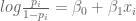
4. Now I summarize my fit to learn about the relationship of previous grade and ACT on the success of the calculus students. I define a grid of ACT scores and consider two sets of covariates corresponding to students who were not successful (0) and successful (1) in precalculs.

act=seq(15,29)
x0=cbind(1,0,act)
x1=cbind(1,1,act)

Then I use the function bprobit.probs to obtain posterior samples of the probability of success in calculus for each set of covariates.

fit.x0=bprobit.probs(x0,fit2)
fit.x1=bprobit.probs(x1,fit2)

I graph the posterior means of the fitted probabilities in the below graph. There are two lines — one corresponding to the students who aced the precalculus class, and another line corresponding to the students who did not ace precalculus.

Several things are clear from this graph. The performance in the precalc class matters — students who ace precalculus have a 30% higher chance of succeeding in the calculus class. On the other hand, the ACT score (that the student took during high school) has essentially no predictive ability. It is interesting that the slopes of the lines are negative, but these clearly isn’t significant.

Bayesian regression

To introduce Bayesian regression modeling, we consider a dataset from De Veaux, Velleman and Bock which collected physical measurements from a sample of 250 males. One is interested in predicting a person’s body fat from his height, waist, and chest measurements.

The file Body_fat.txt contains the data that we read in R.

data=read.table(“Body_fat.txt”,sep=”\t”,header=TRUE)
names(data)
[1] “Pct.BF” “Height” “Waist” “Chest”
attach(data)

Suppose we wish to fit the regression model

Pct.BF ~ Height + Waist + Chest

The standard least-squares fit is done using the lm command in R.

fit=lm(Pct.BF~Height+Waist+Chest)

Here is a portion of the summary of the fit.

summary(fit)

Coefficients:
Estimate Std. Error t value Pr(>|t|)
(Intercept) 2.06539 7.80232 0.265 0.79145
Height -0.56083 0.10940 -5.126 5.98e-07 ***
Waist 2.19976 0.16755 13.129 < 2e-16 ***
Chest -0.23376 0.08324 -2.808 0.00538 **
—
Signif. codes: 0 ‘***’ 0.001 ‘**’ 0.01 ‘*’ 0.05 ‘.’ 0.1 ‘ ’ 1

Residual standard error: 4.399 on 246 degrees of freedom
Multiple R-Squared: 0.7221, Adjusted R-squared: 0.7187
F-statistic: 213.1 on 3 and 246 DF, p-value: < 2.2e-16

Now let’s consider a Bayesian fit of this model. Suppose we place the usual noninformative prior on the regression vector beta and the error variance sigma^2.

g(beta, sigma^2) = 1/sigma^2.

Then there is a simple direct method (outlined in BCUR) of simulating from the posterior distribution of (beta, sigma^2).

1. We first create the design matrix X:

X=cbind(1,Height,Waist,Chest)

The response is contained in the vector Pct.BF.

2. To simulate 5000 draws from the posterior of (beta, sigma), we use the function blinreg in the LearnBayes package.

fit=blinreg(Pct.BF, X, 5000)

The output fit is a list with two components: beta is a matrix of simulated draws of beta where each column corresponds to a sample from component of beta, and sigma is a vector of draws from the marginal posterior of sigma.

We can summarize the simulated draws of beta by computing posterior means and standard deviations.

apply(fit$beta,2,mean)
X XHeight XWaist XChest
1.8748122 -0.5579671 2.2031474 -0.2350661

apply(fit$beta,2,sd)
X XHeight XWaist XChest
7.84069390 0.11050071 0.16839919 0.08286758

Here is a graph of density estimates of simulated draws from the four regression parameters.

par(mfrow=c(2,2))
for (j in 1:4) plot(density(fit$beta[,j]),main=paste(“BETA “,j),
lwd=3, col=”red”, xlab=”PAR”)

What’s so special about Bayesian regression if we are essentially replicating the frequentist regression fit?

We’ll talk about the advantages of Bayesian regression in the next blog posting.

Conditional means prior

In an earlier post, we illustrated Bayesian fitting of a logistic model using a noninformative prior. Suppose instead that we have subjective beliefs about the regression vector. A convenient way of representing these beliefs is by use of a conditional means prior. We illustrate this for our math placement example.

First, we consider the probability p1 that a student in placement level 1 receives an A in the class. Our best guess at p1 is 0.05 and this belief is worth 200 observations — we match this info to a beta(200*0.05, 200*0.95) prior. Next, we consider the probability p5 that a student in level 5 gets an A — our guess at this probability is 0.15 and this guess is worth 200 observations. We match this belief to a beta(200*0.15, 200*0.85) prior. Assuming that our beliefs about p1 and p5 are independent, the joint prior on (p1, p5) is a product of beta densities. Transforming back to the (beta0, beta1) scale, one can show that the prior on beta is given by

g(beta) = p1^a1 (1-p1)^b1 p5^a2 (1-p5)^b2

(Note that the conditional means prior translates to the same functional form as the likelihood where the beta parameters a1, b1, a2, b2 play the role of “prior data”.)

The below figure displays (in red) a sample from the likelihood and (in blue) a sample from the prior. Here we see some conflict between the prior beliefs and the data information about the parameter.