Sale on Bayesian Computation with R

Amazon currently is selling the 2nd edition of Bayesian Computation with R for $14.92 — list price is $59.95.  The package LearnBayes accompanies this text.

Simple Example of Bayesian Learning using LearnBayes

Today I am giving a short course on Bayesian Computation at my stats meeting and I thought it might be helpful to illustrate some basic Bayesian computing if my participants are struggling with the more complicated examples.  This will illustrate some new methods in the “development” version of the LearnBayes package.

Okay, suppose we are interested in estimating a binomial proportion p.  My prior for p is beta(3, 10) and I take a sample of size 10, observing 7 successes and 3 failures.

Defining the log posterior

I write a short R function that defines the log posterior.

 
myposterior <- function(p, stuff){
  dbinom(stuff$y, size=stuff$n, prob=p, log=TRUE) + dbeta(p, stuff$a, stuff$b)
}

I define the inputs (number of successes, sample size, beta shape 1, beta shape 2) by a list d.

 
d <- list(y=7, n=10, a=3, b=10)

I make sure my log posterior function works:

 
myposterior(.5, d)
[1] -1.821714

The R package LearnBayes contains several functions for working with my log posterior — I illustrate some basic ones here.

The function laplace will find the posterior mode and associated variance. The value .4 is a guess at the posterior mode (a starting value for the search).

 
library(LearnBayes)
fit <- laplace(myposterior, .4, d)

In LearnBayes 2.17, I have several methods that will summarize, plot, and simulate the fit.

Summarize the (approximate) posterior:

 
summary(fit)
Var : Mean = 0.696 SD = 0.153

This tells me the posterior for p is approximately normal with mean 0.696 and standard deviation 0.153.

Plot the (approximate) posterior:

 
plot(fit)

This displays the normal approximation to the posterior.

Simulate from the (approximate) posterior:

 
S <- simulate(fit)
hist(S$sample)

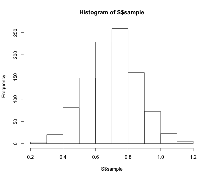
These simulated draws are helpful for performing many types of inferences about p — for example, it would be easy to use these simulated draws to learn about the odds ratio p / (1 – p).

Sequential Learning in Bayes’ Rule

I have pasted the R code for implementing the quality control example I talked about in class

 

########################################################
# Illustration of function bayes to illustrate
# sequential learning in Bayes’ rule
# Jim Albert, August 2013
########################################################

bayes <- function(prior, likelihood, data){
probs <- matrix(0, length(data) + 1, length(prior))
dimnames(probs)[[1]] <- c(“prior”, data)
dimnames(probs)[[2]] <- names(prior)
probs[1, ] <- prior
for(j in 1:length(data))
probs[j+1, ] <- probs[j, ] * likelihood[, data[j]] /
sum(probs[j, ] * likelihood[, data[j]])
dimnames(probs)[[1]] <-
paste(0:length(data), dimnames(probs)[[1]])
data.frame(probs)
}

# quality control example
# machine is either working or broken with prior probs .9 and .1

prior <- c(working = .9, broken = .1)

# outcomes are good (g) or broken (b)
# likelihood matrix gives probs of each outcome for each model

like.working <- c(g=.95, b=.05)
like.broken <- c(g=.7, b=.3)
likelihood <- rbind(like.working, like.broken)

# sequence of data outcomes

data <- c(“g”, “b”, “g”, “g”, “g”, “g”, “g”, “g”, “g”, “b”, “g”, “b”)

# function bayes will computed the posteriors, one datum at a time
# inputs are the prior vector, likelihood matrix, and vector of data

posterior <- bayes(prior, likelihood, data)
posterior

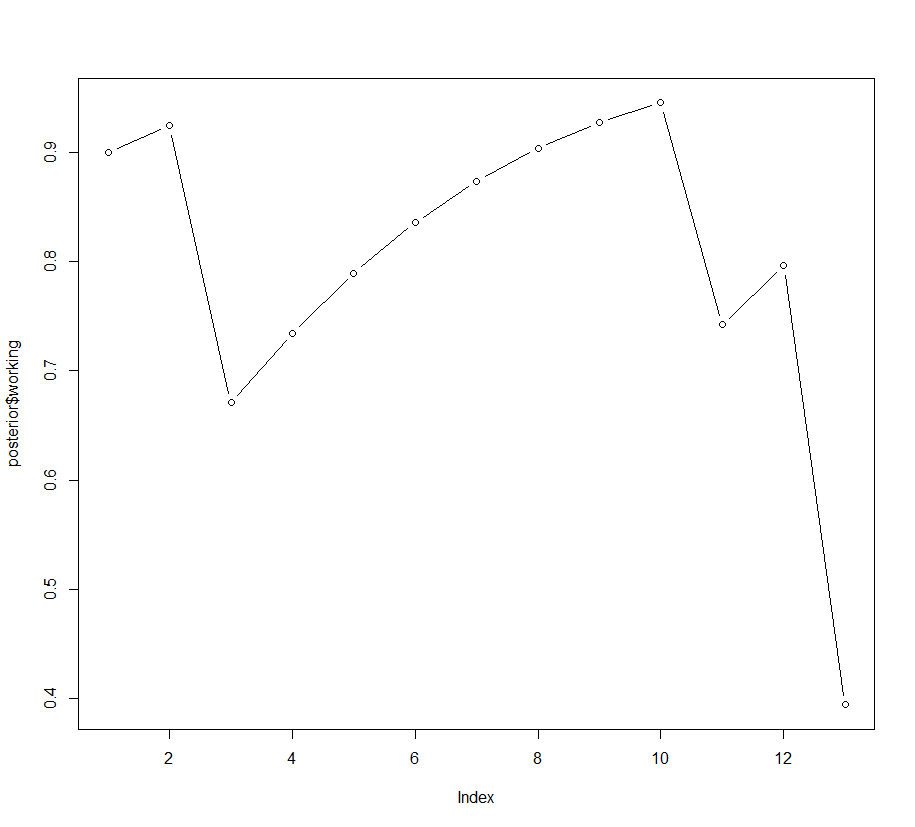
# graph the probs of working as a function of the data observation

plot(posterior$working, type=’b’)

###################################################

Here is the output — the posterior probabilities and the graph.


working broken
0 prior 0.9000000 0.10000000
1 g 0.9243243 0.07567568
2 b 0.6705882 0.32941176
3 g 0.7342373 0.26576271
4 g 0.7894495 0.21055055
5 g 0.8357571 0.16424288
6 g 0.8735119 0.12648812
7 g 0.9035891 0.09641094
8 g 0.9271111 0.07288893
9 g 0.9452420 0.05475796
10 b 0.7420707 0.25792933
11 g 0.7961074 0.20389264
12 b 0.3942173 0.60578268


Graphical elicitation of a beta prior

My students are doing a project where they have to elicit a beta prior for a proportion.  This is a difficult task and any tools to make this process a little easier are helpful.

I’ve been playing with a R package manipulate that is included as part of the RStudio installation (for those who don’t know, RStudio is a nice interface for R).  This package makes it easy to construct sliders, push buttons, and pull-down menus to provide a nice user interface for functions one creates.

Here is a simple illustration of the use of the manipulate package.  One assesses the shape parameters of the beta indirectly by specifying (1) the prior median p.med and (2) the prior 90th percentile p.90.   One inputs values of p.med and p.90 by sliders and you see the beta density curve that matches this information.  I wrote a simple R script that constructs the graph with sliders — the main tools are the manipulate package and the LearnBayes package (the beta.select function).

Here is the script and here is a movie that shows the sliders in action.

 

 

Three Sampling Models for Fire Calls

Continuing our example, suppose our prior beliefs about the mean count of fire calls is Gamma(280, 4).  (Essentially this says that our prior guess at is 70 and the prior standard deviation is about 4.2.)  But we’re unsure about the sampling model — it could be (M1) exponential(), (M2) Poisson(), or (M3) normal with mean and standard deviation 12.

To get some sense about the best sampling model, I’ve plotted a histogram of the fire call counts below.  I’ve overlaid fitted exponential, Poisson, and normal distributions where I estimate by the sample mean.

I think it is pretty clear from the graph that the exponential model is a poor fit.  The fits of the Poisson and normal (sd = 12) models are similar, although I’d give a slight preference to the normal model.

For each model, I compute the logarithm of the predictive probability .   (I wrote a short function defining the log posterior of and then used the laplace function in the LearnBayes package to compute .)

Here are the results:

Model    
————————–
Poisson              -148.0368
exponential        -194.3483
normal(12)        -144.3027
—————————

The exponential model is a clear loser and the Poisson and normal(12) models are close.  The Bayes factor in support of the normal(12) model is

 

Modeling fire alarm counts

Sorry for the long delay since my last post.  It seems that one needs to keep a regular posting pattern, say several days a week. to keep this blog active.

We’re now talking about comparing models by Bayes factors.  To motivate the discussion of plausible models, I found the following website that gives the number of fire calls for each month in Franklinville, NC for the last several years.

Suppose we observe the fire call counts for consecutive months.  Here is a general model for these data.

1. are independent
2. has a prior

Also, suppose we have some prior beliefs about the mean fire count .  We believe that this mean is about 70 and the standard deviation of this guess is 10.

Given this general model structure, we have to think of possible choices for , the sampling density.  We think of the popular distributions, say Poisson, normal, exponential, etc.  Also we should think about different choices for the prior density.   For the prior, there are many possible choices — we typically choose one that can represent my prior information.

Once we decide on several plausible choices of sampling density and prior, then we’ll compare the models by Bayes factors.  To do this, we compute the prior predictive density of the actual data for each possible model.  It is very convenient to perform this calculation for discrete models (where the parameter is discrete) and we’ll first illustrate Bayes factor computations in this special case

Cell phone story — part 3

After talking about this problem in class on Monday, I realized that we don’t understand the texting patterns of undergraduates very well.  So I’m reluctant to specify an informative prior in this situation for the simple reason that I don’t understand this that well.  So I’m going to illustrate using bugs to fit this model using a vague prior.

I have observed the number of text messages for my son for 16 days in this months billing period.  Since his monthly allocation is 5000 messages, I am focusing on the event “number of messages in the 30 days exceeds 5000.”  Currently my son has had 3314 messages and so I’m interested in computing the predictive probability that the number of messages in the remaining 14 days exceeds 1686.

Here I’ll outline using the openbugs software with the R interface in the BRugs package to fit our model.

I’m assuming that you’re on a Windows machine and have already installed the BRugs package in R.

First we write a script that describes the normal sampling model.  Following Kruschke’s Doing Bayesian Data Analysis text, I can enter this model into the R console and write it to a file model.txt.

modelString = ”
model {
for( i in 1:n ){
y[i] ~ dnorm( mu, P )
}
mu ~ dnorm( mu0, P0 )
mu0 <- 100
P0 <- 0.00001
P ~ dgamma(a, b)
a <- 0.001
b <- 0.001
}
”
writeLines(modelString, con=”model.txt”)

# We load in the BRugs package (this includes the openbugs software).

library(BRugs)

# Set up the initial values for and in the MCMC iteration — this puts the values in a file called inits.txt.

bugsInits(list(c(mu = 200, P = 0.05)),
numChains = 1, fileName = “inits.txt”)

# Have openbugs check that the model specification is okay.

modelCheck(“model.txt”)

# Here is our data — n is the number of observations and y is the vector of text message counts.

dataList = list(
n = 16,
y=c(207, 121, 144, 229, 113, 262, 169, 330,
168, 132, 224, 188, 231, 207, 268, 321)
)

# Enter the data into openbugs.

modelData( bugsData( dataList ))

# Compile the model.

modelCompile()

# Read in the initial values for the simulation.

modelInits(“inits.txt”)

# We are going to monitor the mean and the precision.

samplesSet( c(“mu”, “P”))

# We’ll try 10,000 iterations of MCMC.

chainLength = 10000

# Update (actually run the MCMC) — it is very quick.

modelUpdate( chainLength )

# The function samplesSample collects the simulated draws, samplesStats computes summary statistics.

muSample = samplesSample( “mu”)
muSummary = samplesStats( “mu”)

PSample = samplesSample( “P”)
PSummary = samplesStats( “P”)

# From this output, we can compute summaries of any function of the parameters of interest (like the normal standard deviation) and compute the predictive probability of interest.

Let’s focus on the prediction problem.  The variable of interest is z, the number of text messages in the 14 remaining days in the month.  The sampling model assumes that the number of daily text messages is N(), so the sum of text messages for 14 games is N(.

To simulate a single value of z from the posterior predictive distribution, we (1) simulate a value of from its posterior distribution, and (2) simulate z from a normal distribution using these simulated draws as parameters.

Cell phone story — part 2

It is relatively easy to set up a Gibbs sampling algorithm for the normal sampling problem when independent priors (of the conjugate type) are assigned to the mean and precision.  Here we outline how to do this on R.

We start with an expression for the joint posterior of the mean and the precision :

(Here S is the sum of squares of the observations about the mean.)

1.  To start, we recognize the two conditional distributions.

• The posterior of given is given by the usual updating formula for a normal mean and a normal prior.  (Essentially this formula says that the posterior precision is the sum of the prior and data precisions and the posterior mean is a weighted average of the prior mean and the sample mean where the weights are proportional to the corresponding precisions.
• The posterior of given has a gamma form where the shape is given by and the scale is easy to pick up.

2.  Now we’re ready to use R.  I’ve written a short function that implements a single Gibbs sampling cycle.  To understand the code, here are the variables:

– ybar is the sample mean, S is the sum of squares about the mean, and n is the sample size
– the prior parameters are (mu0, tau) for the prior and (a, b) for the precision
– theta is the current value of ()

The function performs the simulations from the distributions [] and and returns a new value of ()

one.cycle=function(theta){
mu = theta[1]; P = theta[2]
P1 = 1/tau0^2 + n*P
mu1 = (mu0/tau0^2 + ybar*n*P) / P1
tau1 = sqrt(1/P1)
mu = rnorm(1, mu1, tau1)

a1 = a + n/2
b1 = b + S/2 + n/2*(mu – ybar)^2
P = rgamma(1, a1, b1)
c(mu, P)
}

All there is left in the programming is some set up code (bring in the data and define the prior parameters), give a starting value, and collect the vectors of simulated draws in a matrix.

Cell phone story

I’m interested in learning about the pattern of text message use for my college son.  I pay the monthly cell phone bill and I want to be pretty sure that he won’t exceed his monthly allowance of 5000 messages.

We’ll put this problem in the context of a normal distribution inference problem.  Suppose , the number of daily text messages (received and sent) is normal with mean and standard deviation .  We’ll observe , the number of text messages in the first 13 days in the billing month.  I’m interested in the predictive probability that the total of the count of text message in the next 17 days exceeds 5000.

We’ll talk about this problem in three steps.

1. First I talk about some prior beliefs about that we’ll model by independent conjugate priors.
2.  I’ll discuss the use of Gibbs sampling to simulate from the posterior distribution.
3. Last, we’ll use the output of the Gibbs sampler to get a prediction interval for the sum of text messages in the next 17 days.

Here we talk about prior beliefs.  To be honest, I didn’t think too long about my beliefs about my son’s text message usage, but here is what I have.

1. First I assume that my prior beliefs about the mean and standard deviation of the population of text messages are independent.  This seems reasonable, especially since it is easier to think about each parameter separately.
2. I’ll use conjugate priors to model beliefs about each parameter.  I believe my son makes, on average, 40 messages per day but I could easily be off by 15.  So I let .
3. It is harder to think about my beliefs about the standard deviation of the text message population.   After some thought, I decide that my prior mean and standard deviation of are 5 and 2, respectively.  We’ll see shortly that it is convenient to model the precision by a distribution.  It turns out that is a reasonable match to my prior information about .

In the next blog posting, I’ll illustrate writing a R script to implement the Gibbs sampling.

Learning from the extremes – part 3

Continuing our selected data example, suppose we want to fit our Bayesian model by using a MCMC algorithm.  As described in class, the Metropolis-Hastings random walk algorithm is a convenient MCMC algorithm for sampling from this posterior density.  Let’s walk through the steps of doing this using LearnBayes.

1.  As before, we write a function minmaxpost that contains the definition of the log posterior.  (See an earlier post for this function.)

2.  To get some initial ideas about the location of (), we use the laplace function to get an estimate at the mean and variance-covariance matrix.

data=list(n=10, min=52, max=84)
library(LearnBayes)
fit = laplace(minmaxpost, c(70, 2), data)
mo = fit$mode
v = fit$var

Here mo is a vector with the posterior mode and v is a matrix containing the associated var-cov matrix.

Now we are ready to use the rwmetrop function that implements the M-H random walk algorithm.  There are four inputs:  (1) the function defining the log posterior, (2) a list containing var, the estimated var-cov matrix, and scale, the M-H random walk scale constant, (3) the starting value in the Markov Chain simulation, (4) the number of iterations of the algorithm, and (5) any data and prior parameters used in the log posterior density.

Here we’ll use v as our estimated var-cov matrix, use a scale value of 3, start the simulation at and try 10,000 iterations.

s = rwmetrop(minmaxpost, list(var=v, scale=3), c(70, 2), 10000, data)

I display the acceptance rate — here it is 19% which is a reasonable value.

> s$accept
[1] 0.1943

Here we can display the contours of the exact posterior and overlay the simulated draws.

mycontour(minmaxpost, c(45, 95, 1.5, 4), data,
          xlab=expression(mu), ylab=expression(paste("log ",sigma)))
points(s$par)

It seems like we have been successful in getting a good sample from this posterior distribution.