Robust modeling

The Phillies are still alive in the World Series and so I’m allowed to continue to talk about baseball.

In the situation where we observe a sample of measurement data , a common assumption to assume that they are a random sample from a normal population with mean and standard deviation .  But sometimes this assumption is inappropriate.  One measure of hitting effectiveness is the OBP, the proportion of time that a hitter gets on base.  I collected the OBPs (actually 1000 x OBP) for a group of 24 players who played for the west coast NL teams (Dodgers, Giants, and Padres) in the 2004 season.  Here’s a jittered dotplot of the OBPs:

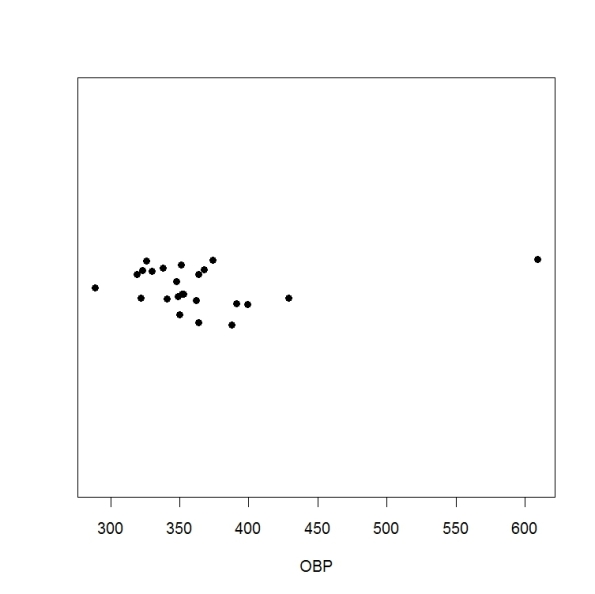
Clearly, a normal population is inappropriate here since we have one obvious outlier — Barry Bonds in that season had an usually large OBP of 609.

In many situations, it makes more sense to assume that are distributed from a “flat-tailed” distribution where outliers are more likely to occur.  One example of a flat-tailed distribution is the t form that depends on a location , a scale and a degrees of freedom .  Here we assume a small value of the degrees of freedom and focus on estimating .

This is an attractive way of fitting a t sampling model.  First, a t distribution can represented as a scale mixtures of normals.  Suppose we let be distributed normal with mean and variance , and then we let the parameter be distributed Gamma with shape and rate .  When you integrate out , one sees this is equivalent to assuming is N(.

Suppose we use this scale mixture representation for each observation.  We can write this as a hierarchical model:

1.   is distributed N()

2. is distributed Gamma ()

3. has the prior .

In class, we’ll show that can sample from this model easily using Gibbs sampling.  This algorithm is implemented using the function in the LearnBayes package.

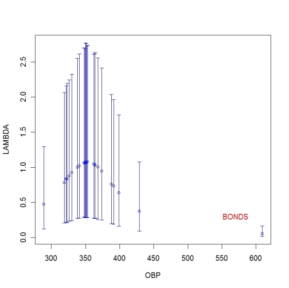
The posteriors of the extra scale parameters are of interest, since they reflect the influence of the th observation on the estimation of the mean and variance.  Below I display error bars that show 90% interval estimates for each of the for my OBP example.  Note that the posterior for the scale parameter for Barry Bonds is concentrated near 0.  This is reasonable, since it is desirable to downweight the influence of Bonds OBP in the estimation of, say, the average OBP.

Home run hitting — priors?

At our department’s colloquium last week, there was an interesting presentation on the use of an exchangeable prior in a regression context.  The analysis was done using WinBUGS using some standard choices of “weekly informative” priors.  That raises the natural question — how did you decide on this prior?

Let’s return to the home run hitting example where an exchangeable prior was placed on the set of home run hitting probabilities.  We assumed that were iid and then the hyperparameters and were assumed independent where was assigned the prior and was assigned the log logistic form .

When I described these priors, I just said that they were “noninformative” and didn’t explain how I obtained them.

The main questions are:

1.  Does the choice of vague prior matter?
2.  If the answer to question 1 is “yes”, what should we do?

When one fits an exchangeable model, one is shrinking the observed rates towards a common value.  The posterior of tells us about the common value and the posterior of tells us about the degree of shrinkage.  The choice of vague prior for is not a concern — we can assume is uniform or distributed according to the improper prior .   However, the prior on can be a concern.  If one assigns the improper form , it can be shown that the posterior may be improper.  So in general one needs to assign a proper prior to .  One convenient choice is to assume that has a logistic density with location and scale .  In my example, I assumed that .

Since I was arbitrary in my choice of parameters for this logistic prior on , I tried different choices for and .  I tried values of between -4 and 4 and values of between 0.2 and 10.  What did I find?  The posterior mode of stayed in the 4.56 – 4.61 range for all of the priors I considered.  In this example, we have data from 605 players and clearly the likelihood is driving the inference.

What if the choice of and does matter?  Then one has to think more carefully about these parameters.  In this baseball context, I am pretty familiar with home run hitting rates.  Based on this knowledge, I have to figure out a reasonable guess at the variability of the home run probabilities that would give me information about .

 

Home run rates — prediction

Last post, we illustrated fitting an exchangeable model on home run hitting probabilities for all players (non pitchers) in the 2007 season.

But actually, teams aren’t really interested in estimating hitting probabilities.  They are primarily interested in predicting a player’s home run performance the following 2008 baseball season.

We already have the posterior distribution for the 2007 home run probabilities.  Assuming that the probabilities stay the same for the following season and that the players will have the same number of at-bats, we can easily predict their 2008 home run counts from the posterior predictive distribution.

For each player, I simulated the predictive distribution of the number of home runs in at-bats in the 2008 season.  I summarize each distribution by its mode — this is the most probable value of from the predictive distribution.

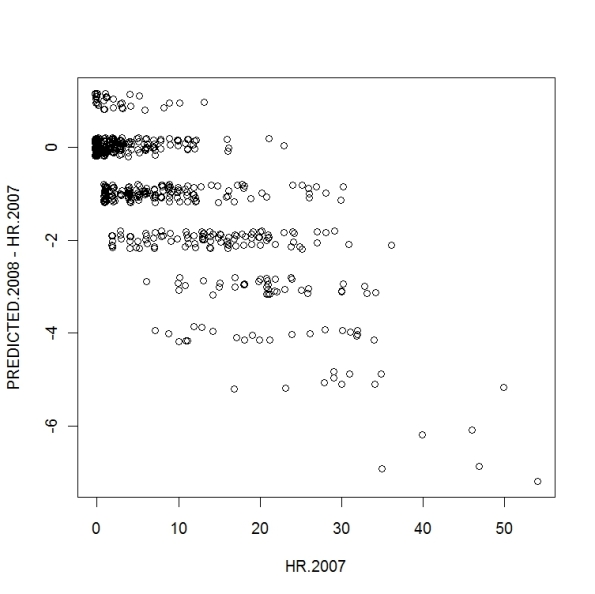
In the first graph, for all players I plot the number of 2007 home runs (horizontal) against the predicted number of 2008 home runs – the number of 2007 home runs (vertical).   Given the 2007 home run count, I’m interested in my prediction of the change to the following season.  (I jittered the points so you can see the individual observations.)  For the weak home run hitters (on the left side of the graph), I predict they will perform a little worse or better the following season.  But for the heavy hitters, I predict they will hit 5-7 home runs worse in the 2008 season.  Generally, there is a negative slope in the graph that illustrates the “regression to the mean” effect.

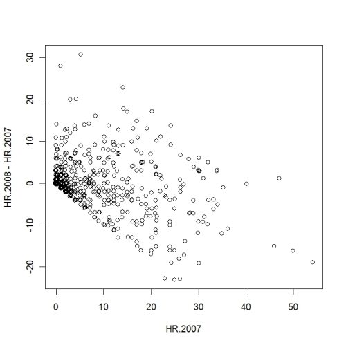
Since we have the actual 2008 home run counts, we can actually compare the 2007 and 2008 counts to see if there is a similar effect.  In the following graph, I plot the 2007 counts against the change (2008 count – 2007 count). What do we see?  There is a negative correlation as we suspected.  Hitters who did well in 2007 tended to get worse in 2008, and a number of light hitters in 2007 tended to do better in 2008.  The biggest difference between the actual data and our predictions is the magnitude of the changes.  Three of the top hitters, for example, hit 15-20 home runs in 2008.

 

Home run rates — fitting an exchangeable model

Continuing our home run hitting example, we observe home run counts where is distributed . Suppose we assign the home run probabilities the following exchangeable model.

1.   distributed

2. independent, distributed distributed .

We described the computing strategy in class to summarize the posterior distribution of .  We find

1.  For , the posterior median is 0.0283 and a 90% interval estimate is (.0268, .0296).

2. For , the posterior median is 99 and a 90% interval estimate is (85, 116).

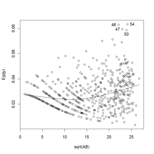
We find posterior means for the home run probabilities .  We plot the posterior means against the square root of the at-bats for the 605 non-pitchers.

This is a very different graph pattern compared to the figure plotting sqrt(AB) against the observed home run rates.  Several things to note.

1.  For the players with few AB, their home run rates are strongly shrunk towards the overall home run rate.  This is reasonable — we have little information about these players’ true home run hitting abilities.

2.  Who are the best home run hitters?  It is clear from the figure that four hitters stand out — they are the ones in the upper right corner of the graph that I’ve labeled with the number of home runs.  The best home run hitters, that is the ones with the highest estimated home run probabilities, are the two player with 46 and 54 at-bats.

3.  I’ve drawn a smoothing curve to indicate the main pattern in the graph.  Note that it’s an increasing curve — this means that players with more AB tend to have higher home run probabilities.  This makes sense — the better hitters tend to get more playing time and more at-bats.

Estimating home run rates

Since the World Series starts tomorrow, it seems appropriate to use baseball data to illustrate hierarchical modeling.

I collected home run for all nonpitchers in the 2007 baseball season.  We observe the pair , the number of home runs and the number of at-bats (opportunities) for the th player.

Who was the best home run hitter this season?  Major League Baseball’s criteria is simply the number of home runs hit.  Alex Rodriquez hit the most home runs  (54) that season.

Was A-Rod the best home run hitter in 2007?  Since the number of at-bats varies among players, maybe it makes more sense to consider the player who had the highest home run rate RATE = HR/AB.

Who had the highest home run rate in the 2007 season?  Actually, it was Charlton Jimerson who had 1 home run in 2 at-bats for a home run RATE = 1/2 = 0.500.

Should Jimerson be given the home run hitting crown?  Of course not, since he had only two at-bats.  It makes more sense to restrict our attention to hitters who had more opportunities.  But how many opportunities (AB) is enough?

Below I’ve plotted the home run rate HR/AB against the square root of the number of AB for all nonpitchers in the 2007 season.

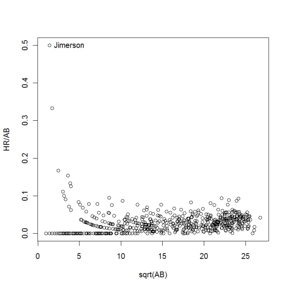
This figure dramatically illustrates the problem of interpreting a collection of rates when the sample sizes vary.  The home run rates are much more variable for small sample sizes.  If one wishes to simultaneously estimate the probabilities of a home run for all players, it seems desirable to adjust the small sample rates towards the average rate.  We’ll see that we can accomplish this by means of an exchangeable prior model.

Modeling airline on-time arrival rates

I am beginning to teach a new course on multilevel modeling using a new book by Gelman and Hill.

Here is a simple example of multilevel modeling. The Department of Transportation in May 2007 issued the Air Travel Consumer Report designed to give information to consumers regarding the quality of services of the airlines. For 290 airports across the U.S., this report gives the on-line percentage for arriving flights. Below I’ve plotted the on-line percentage against the log of the number of flights for these airlines.
What do we notice in this figure? There is a lot of variation in the on-time percentages. Also there variation in the on-line percentages seems to decrease as the number of flights increases.

What explains this variation? There are a couple of causes. First, there are genuine differences in the quality of service at the airports that would cause differences in on-time performance. But also one would expect some natural binomial variability. Even if a particular airport ‘s planes will be on-time 80% in the long-run, one would expect some variation in the on-time performance of the airport in a short time interval.

In multilevel modeling, we are able to isolate the two types of variation. We are able to model the binomial variability and also model the differences between the true on-time performances of the airports.

To show how multilevel model estimates behavior, I’ve graphed the estimates in red in the following graph.

I call these multilevel estimates “bayes” in the figure. Note that there are substantial differences between the basic estimates and the multilevel estimates for small airports with a relatively small number of flights.

Gibbs Sampling for Hierarchical Models

Gibbs sampling is an attractive “automatic” method of setting up a MCMC algorithm for many classes of models. Here we illustrate using R to write a Gibbs sampling algorithm for the normal/normal exchangeable model.

We write the model in three stages as follows.

1. The observations y1, …, yk are independent where yj is N(thetaj, sigmaj^2), where we write N(mu, sigma2) to denote the normal density with mean mu and variance sigma2. We assume the sampling variances sigma1^2, …, sigmak^2 are known.

2. The means theta1,…, thetak are a random sample from a N(mu, tau2) population. (tau2 is the variance of the population).

3. The hyperparameters (mu, tau) are assumed to have a uniform distribution. This implies that the parameters (mu, tau2) have a prior proportional to (tau2)^(-1/2).

To write a Gibbs sampling algorithm, we write down the joint posterior of all parameters (theta1, …, thetak, mu, tau2):

From this expression, one can see

1. The posterior of thetaj conditional on all remaining parameters is normal, where the mean and variance are given by the usual normal density/normal prior updating formula.

2. The hyperparameter mu has a normal posterior with mean theta_bar (the sample mean of the thetaj) and variance tau2/k.

3. The hyperparameter tau2 has an inverse gamma posterior with shape (k-1)/2 and rate 1/2 sum(thetaj – mu)^2.

Given that all the conditional posteriors have convenient functional forms, we write a R function to implement the Gibbs sampling. The only inputs are the data matrix (columns containing yj and sigmaj^2) and the number of iterations m.

I’ll display the function normnormexch.gibbs.R with notes.

normnormexch.gibbs=function(data,m)
{
y=data[,1]; k=length(y); sigma2=data[,2] # HERE I READ IN THE DATA

THETA=array(0,c(m,k)); MU=rep(0,m); TAU2=rep(0,m) # SET UP STORAGE

mu=mean(y); tau2=median(sigma2) # INITIAL ESTIMATES OF MU AND TAU2

for (j in 1:m) # HERE’S THE GIBBS SAMPLING
{
p.means=(y/sigma2+mu/tau2)/(1/sigma2+1/tau2) # CONDITIONAL POSTERIORS
p.sds=sqrt(1/(1/sigma2+1/tau2)) # OF THETA1,…THETAK
theta=rnorm(k,mean=p.means,sd=p.sds)

mu=rnorm(1,mean=mean(theta),sd=sqrt(tau2/k)) # CONDITIONAL POSTERIOR OF MU

tau2=rigamma(1,(k-1)/2,sum((theta-mu)^2)/2) # CONDITIONAL POSTERIOR OF TAU2

THETA[j,]=theta; MU[j]=mu; TAU2[j]=tau2 # STORE SIMULATED DRAWS
}
return(list(theta=THETA,mu=MU,tau2=TAU2)) # RETURN A LIST WITH SAMPLES
}

Here is an illustration of this algorithm for the SAT example from Gelman et al.

y=c(28,8,-3,7,-1,1,18,12)
sigma=c(15,10,16,11,9,11,10,18)
data=cbind(y,sigma^2)
fit=normnormexch.gibbs(data,1000)

In the Chapter 7 exercise that used this example, a different sampling algorithm was used to simulate from the joint posterior of (theta, mu, tau2) — it was a direct sampling algorithm based on the decomposition

[theta, mu, tau2] = [mu, tau2] [theta | mu, tau2]

In a later posting, I’ll compare the two sampling algorithms.

A Prediction Contest

Concluding our baseball example, recall that we observed the home run rates for 20 players in the month of April and we were interested in predicting their home run rates for the next month. Since we have collected data for both April and May, we can check the accuracy of three prediction methods.

1. The naive method would be to simply use the April rates to predict the May rates. Recall that the data matrix is d where the first column are the at-bats and the second column are the home run counts.

pred1=d[,2]/d[,1]

2. A second method, which we called the “pooled” method, predicts each player’s home run rate by the pooled home run rate for all 20 players in April.

pred2=sum(d[,2])/sum(d[,1])

3. The Bayesian method, predicts a player’s May rate by his posterior mean of his true rate lambda_j.

pred3=post.means

One measure of accuracy is the sum of absolute prediction errors.

The May home run rates are stored in the vector may.rates. We first compute the individual prediction errors for all three methods.

error1=abs(pred1-may.rates)
error2=abs(pred2-may.rates)
error3=abs(pred3-may.rates)

We use the apply statement to sum the absolute errors.

errors=cbind(error1,error2,error3)
apply(errors,2,sum) # sum of absolute errors for all methods

error1 error2 error3
0.3393553 0.3111552 0.2622523

By this criterion, Bayes beats Pooled beats Naive.

Finally, suppose we are interested in predicting the number of home runs hit by the first player Chase Utley in May. Suppose we know that he’ll have 115 at-bats in May.

1. We have already simulated 10,000 draws from Utley’s true home run rate lambda1 — these are stored in the first column of the matrix lam vector.

2. Then 10,000 draws from Utley’s posterior predictive distribution are obtained by use of the rpois function.

ys1=rpois(10000,AB*lam[,1])

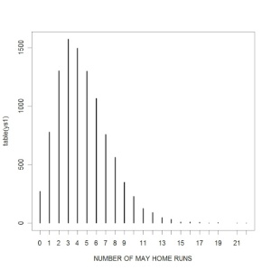
We graph this predictive distribution by the command

plot(table(ys1),xlab=”NUMBER OF MAY HOME RUNS”)

The most likely number of May home runs is 3, but a 90% prediction interval is [1, 9].

Fitting an Exchangeable Model

Continuing our baseball example, we observe yi home runs in ei at-bats for the ith player. We assume

1. y1, …, y20 are independent, yi is Poisson(lambda_i)
2. the true rates lambda_1,…, lambda_20 are independent Gamma(alpha, alpha/mu)
3. the hyperparameters alpha, mu are independent, mu is distributed 1/mu, alpha is distributed according to the proper prior z0/(alpha+z0)^2, where z0 is the prior median

The data is stored as a matrix d, where the first column are the ei and the second column are the yi. In our example, we let z0 = 1; that is, the prior median of alpha is one.

Here is our computing strategy.

1. First we learn about the hyperparameters (alpha, mu). The posterior of (log alpha, log mu) is programmed in the LearnBayes function poissgamexch. Here is a contour plot.

ycontour(poissgamexch,c(-1,8,-4.2,-2.5),datapar)
title(xlab=”LOG ALPHA”,ylab=”LOG MU”)

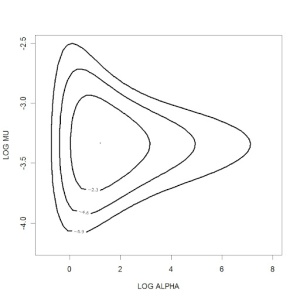
We use the function laplace to find the posterior mode and associated variance-covariance matrix. The output from laplace is used to find a proposal variance and scale parameter to use in a random walk Metropolis chain. We simulate 10,000 draws from the posterior of (log alpha, log mu). (This chain has approximately a 30% acceptance rate.)

fit=laplace(poissgamexch,c(2,-3.2),datapar)
proposal=list(var=fit$var,scale=2)
mcmcfit=rwmetrop(poissgamexch,proposal,c(1,-3),10000,datapar)

By exponentiating the simulated draws from mcmcfit, we get draws from the marginal posteriors of alpha and mu. We draw a density plot of alpha and superimpose the prior density of alpha.

alpha=exp(mcmcfit$par[,1])
mu=exp(mcmcfit$par[,2])
plot(density(alpha,adjust=2),xlim=c(0,20),col=”blue”,lwd=3,xlab=”ALPHA”,
main=”POSTERIOR OF ALPHA”)

prior=function(alpha,z0) z0/(alpha+z0)^2
theta=seq(.0001,20,length=200)
lines(theta,prior(theta,1),col=”red”,lwd=3)

2. Now we can learn about the true rate parameters. Conditional on hyperparameter values, lambda_1, …, lambda_20 have independent gamma posteriors.

We write a short function to simulate draws of lambda_j for a particular player j.

trueratesim=function(j,data,alpha,mu)
{
e=data[,1]; y=data[,2]
rgamma(length(alpha),shape=alpha+y[j],rate=alpha/mu+e[j])
}

Then we can simulate draws of all the true rates by use of the sapply function.

lam=sapply(1:20,trueratesim,d,alpha,mu)

The output lam is a 10,000 by 20 matrix. We can compute posterior means by the apply function.

post.means=apply(lam,2,mean)

To show the behavior of the posterior means, we draw a plot where
(1) we show the observed rates yi/ei as red dots
(2) we show the posterior means as blue dots
(3) a horizontal line is draw at the mean home run rates for all 20 players.

Predicting home run rates

Here is a simple prediction problem. Suppose we observe the number of home runs and the number of at-bats for 20 baseball players during the first month of the baseball season (April).

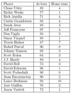We observe corresponding home run rates: Utley 4/88, Weeks 1/77, Aurila 4/71, and so on.

From this data, we want to predict the home run rates for the same 20 players for the next month (May).

How can we best do this? Here are some opening comments.

1. One idea would be to estimate the May rates just by using the April rates. So we predict Utley’s May rate to be 4/88, Weeks rate to be 1/77, etc. This may not be a good idea since we have limited data for each player.

2. Or maybe a better strategy would be to combine the data. Collectively in April, this group hit 60 home runs in 1697 at-bats for a rate of 60/1697 = 0.035. We could estimate each player’s May rate by 0.035. But this would ignore the fact that players have different abilities to hit home runs.

3. Actually, the best prediction strategy is a compromise between the first two ideas. A good plan is to predict a player’s May rate by a “shrinkage” estimate that shrinks a player’s individual rate towards the combined rate.

In the following postings, we’ll illustate how to fit a Bayesian exchangeable model to these data that gives a good prediction strategy.