Modeling Field Goal Kicking

Since it is (American) football season, it seemed appropriate to do a football example to illustrate summarizing a bivariate posterior.

One way of scoring points in football is by kicking field goals.  The ball is lined up at a particular location on the field and the kicker attempts to kick the ball through the uprights.

We are interested in looking at the relationship between the distance of the attempt (in yards) and the result of the kick (success and failure).  I collect the results of 31 field goal attempts for the Big Ten college games in the second week of the 2011 season.   I read the data into R from the class web folder and display the beginning of the data frame fieldgoal:

> fieldgoal=read.csv("http://personal.bgsu.edu/~albert/MATH6480/DATA/fieldgoal.csv")
> head(fieldgoal)
  Distance Result
1       42      1
2       54      1
3       20      1
4       42      0
5       50      1
6       38      0

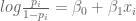
A logistic model can be used to represent this data.  Let denote the result of the th kick at distance — either the kick is good () or it is missed ().  Let denote the probability that .  A simple logistic model says that

The standard way of fitting this model is based on maximum likelihood based on the iterative reweighted least-squares algorithm.  We can implement this algorithm using the R glm function with the family = binomial argument.

> glm(Result ~ Distance, family = binomial, data = fieldgoal)

Coefficients:
(Intercept)     Distance
    3.81329     -0.07549

As expected, the slope is negative — this means that it is harder to make a field goal for a longer distance.

We’ll use this example in a future post to illustrate prior modeling and “brute force” computation of the posterior.