Prediction problem

In class, I described a simple Bayesian prediction problem.  One observes the number of fire calls in a small California city for 30 days — the total number of fire calls in this period is 158.  An administrator is interested in predicting the total number of calls in the next seven days.

We assume that y, the number of calls in a day, is Poisson with mean .  Suppose our prior beliefs about are described by a normal density with mean 10 and standard deviation 2.

I first write a simple function compute.post that computes and plots the posterior (using the likelihood times prior recipe) on a grid between lo and hi.
compute.post=function(lo, hi,...){
lambda = seq(lo, hi, length=100)
prior = dnorm(lambda, 10, 2)
like = lambda^158 * exp(-30*lambda)
post = prior * like
plot(lambda, post,...)
list(L = lambda, P = post)
}

With some trial and error, the interval (3.3, 7.5) seems to bracket the posterior well.

S=compute.post(3.3, 7.5, type="l", col="red")

Next I take a simulated sample from the posterior by using the sample function.

sim.lambda = sample(S$L, 1000, replace=TRUE, prob=S$P)

Last, I simulate a sample from the posterior predictive density of z, the number of fire calls in seven days.  Since [z | ] is Poisson(7 , we simulate z by (1) simulating from the posterior and (2) simulating z from a Poisson(7 ) distribution.  This is easy to do by using the vector properties of the random simulation functions.

sim.z = rpois(1000, 7*sim.lambda)

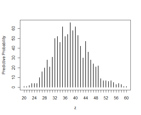
Here is a graph of the predictive distribution (by tabulating and plotting the simulated values of z).

Brute force Bayes for one parameter

Although we talk a lot about conjugate analyses, one doesn’t need to restrict oneself to the use of conjugate priors.  Here we illustrate learning about a Poisson mean using a normal prior on the mean .

Suppose I observe the following number of fire calls for a particular community each week:  0, 0, 1, 3, 2, 2.  If we assume , the number of fire calls in week , is Poisson(), then the likelihood function is given by

Suppose I represent my prior beliefs about by a normal curve with mean 3 and standard deviation 1.  Then the posterior is given by (up to an unknown proportionality constant) by

Here is a simple brute-force method of summarizing this posterior.

1.  Choose a grid of values that covers the region where the posterior is concentrated (this might take some trial and error).

2.  On this grid, compute the prior, likelihood, and posterior.

3.  Using the R sample function, take a large sample from the grid where the probabilities of the points are proportional to the like x prior values.

4.  Summarize this posterior simulated sample to learn about the location of the posterior.

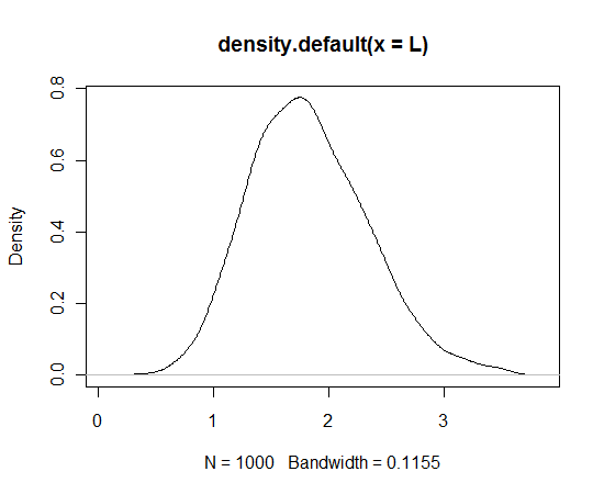
Here’s some R code for this example.  I use the plot function to make sure the grid does cover the posterior.  The vector L contains 1000 draws from the posterior.

lambda = seq(0, 5, by=0.1)
like = exp(-6*lambda)*lambda^8
prior = dnorm(lambda, 3, 1)
post = like * prior
plot(lambda, post)
L = sample(lambda, size=1000, prob=post, replace=TRUE)
plot(density(L))  # density graph of simulated draws

Poisson mean example, part II

In the last post, I described the process of determining a prior for , my son’s average number of text messages per day.   I decided to model my beliefs with a gamma(a, b) density with a = 44.4 and b = 4.4.

Now I observe some data.  I looked at the online record of text messaging for the first seven days that’s been at school and observe the counts

Sat  Sun  Mon  Tue  Wed  Thu  Fri
19     4      26      17    15       0    17

If we assume these counts are Poisson with mean , then the likelihood function is given by

L(lambda) =  lambda^s  exp(-n lambda),

where is the number of observations (7) and is the sum of the observations ( 98).

The posterior density (using the prior times likelihood recipe) is given by

L(lambda) x g(lambda) = lambda^{a+s-1}  exp(-(b+n) lambda),

which we recognize as a gamma density with shape and rate .

Using the following R commands, we construct a triplot (prior, likelihood, and posterior).

> a=44.4; b=4.4

> s=sum(y); n=length(y)

> a=44.4; b=4.4
> s=sum(y); n=length(y)
> curve(dgamma(x,shape=s+a,rate=n+b),col=”red”,xlab=”LAMBDA”,
+   ylab=”DENSITY”,lwd=3,from=3,to=25)
> curve(dgamma(x,shape=a,rate=b),col=”blue”,lwd=3,add=TRUE)
> curve(dgamma(x,shape=s+1,rate=n),col=”green”,lwd=3,add=TRUE)
> legend(“topright”,c(“PRIOR”,”LIKELIHOOD”,”POSTERIOR”),
+  col=c(“blue”,”green”,”red”),lty=1,lwd=3)

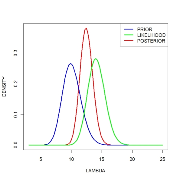Note that (1) the posterior is a compromise between the data information (likelihood) and the prior  and (2) the posterior is more precise since we are combining two sources of information.

I would like to predict my son’s text message use in the next month.  Let denote the number of text messages in the next month.  The total number of messages has, conditional on , a Poisson distribution with mean .

I am interested in computing the posterior predictive  distribution for .  One can simulate this distribution by (1) simulating a value of the parameter from the gamma(142.4, 11.4) posterior and then (2) simulating from a Poisson distribution with mean .

We can do this simulation in R in two lines.   In the last line, I tabulate the values of and plot the counts.

> lambda=rgamma(1000,shape=142.4,rate=11.4)
> ys=rpois(1000,30*lambda)
> plot(table(ys),ylab=”FREQUENCY”)

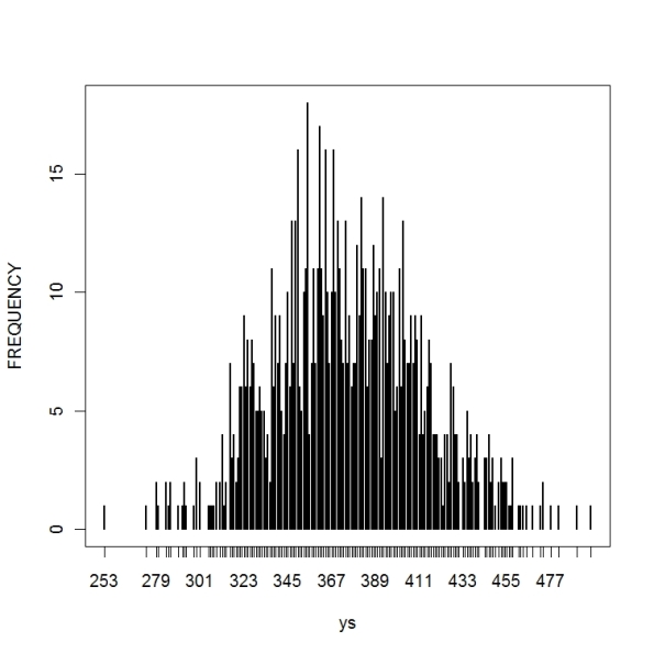Looking at the graph, it is likely that my son will have between 310 and 450 text messages in the next 30 days.

Constructing a prior for a Poisson mean

I am interested in learning about my son’s cell phone use.   Suppose the mean number of text messages that he sends and receives per day is equal to .   I will observe the number of text messages for days — we’ll assume that conditional on , are independent Poisson().

How do I construct a prior density on ?   Suppose I model my beliefs by use of a gamma density with shape parameter and rate parameter .  I want to figure out the values of the prior parameters and .

There are two distinct ways of assessing your prior.  One can think about plausible values of the mean number of daily text messages .  Alternatively, it may be easier to think about the actual number of text messages — if we assume a gamma prior, then one can show that the predictive density of is given by

Personally, I think it is easier to think about the number of text messages .  My best prediction at is 10.  After some additional thought, I decide that my standard deviation for is equal to 3.5.    One can show that the mean and standard deviation of the predictive density are given by

If one matches my guesses with these expressions, one can show .

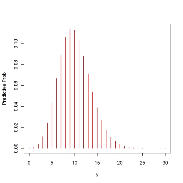
To see if these values make any sense, I plot my predictive density.  This density is a special case of a negative binomial density where (using the R notation)

size = a,  prob = b /(b + 1).

I graph using the following R commands.  One can compute P(5 <= y <= 15) = 0.89 which means that on 89% of the days, I believe Steven will send between 5 and 15 messages.

a = 44.4; b = 4.4

plot(0:30,dnbinom(0:30,size=a,prob=b/(b+1)),type=”h”,

xlab=”y”, ylab=”Predictive Prob”, col=”red”, lwd=2)

a = 44.4; b = 4.4
plot(0:30,dnbinom(0:30,size=a,prob=b/(b+1)),type=”h”,
xlab=”y”, ylab=”Predictive Prob”, col=”red”, lwd=2)

Modeling with Cauchy errors

One attractive feature of Bayesian thinking is that one can consider alternative specifications for the sampling density and prior and these alternatives makes one think more carefully about the typical modeling assumptions.

Generally we observe a sample distributed from a sampling density depending on a parameter .  If we assign  a prior density , then the posterior density is given (up to a proportionality constant) by

Consider the following Cauchy/Cauchy model as an alternative to the usual Normal/Normal model.  We let be distributed from a Cauchy density with location and known scale parameter , and we assign a Cauchy prior with location and scale .

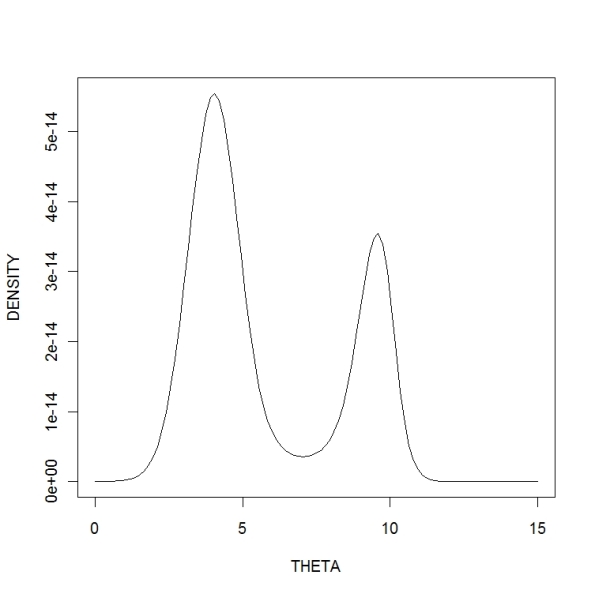
Of course, this is not going to be a conjugate analysis — the posterior density has a complicated form.  But it is easy to use R to plot and summarize the posterior density.

First we define the posterior density for .  The arguments to the function are theta (which could be a vector), the vector of data values, the known scale parameter , and the prior parameters andn .  The output is a vector of values of the (unnormalized) posterior density.

posterior=function(theta,data,scale,mu0,tau)

{

f=function(theta) prod(dcauchy(data,theta,scale))

likelihood=sapply(theta,f)

prior=dcauchy(theta, mu0, tau)

return(prior*likelihood)

}

posterior=function(theta,data,scale,mu0,tau)
{
f=function(theta) prod(dcauchy(data,theta,scale))
likelihood=sapply(theta,f)
prior=dcauchy(theta, mu0, tau)
return(prior*likelihood)
}

(This function is a little tricky to program since both theta and data are vectors.)

We can plot the posterior density using the curve function.   We first give the data vector, assume and assign a Cauchy(0, 1) prior for .

data=c(2,5,4,3,10,11,10,9)

We then use the curve function to plot the posterior.  After some preliminary work, we know that the probability mass falls between 0 and 15, so we use from = 0, to = 15 in the function.

curve(posterior(x,data,1,0,1),from=0,to=15,xlab=”THETA”,ylab=”DENSITY”)

Here is the plot that is produced.  Note the interesting bimodal shape.  One can obtain different posterior shapes when we model using Cauchy densities.  (Question:  Why does the posterior have this particular shape?)

How many more home runs will Ryan Howard hit?

Here is a basic proportion problem.  We are approaching the end of the 2009 baseball season and Ryan Howard of the Philadelphia Phillies currently has 38 home runs in 540 at-bats (opportunities).  I project that he will have 85 more at-bats this season.  How many additional home runs will he hit?

Let p be the probability that Howard hits a home run in a single at-bat during the 2009 season.  We’ll address this prediction problem in three steps.  First, we’ll use past data from previous seasons to form a prior distribution for p.  Second, we’ll update our beliefs about p using the 2009 data.  Last, we’ll predict the number of future at-bats from the posterior predictive distribution.  In this process, we’ll illustrate the use of some functions from the LearnBayes package in R.

1.  My prior.

In the four previous seasons (2005 through 2008) his home runs/at-bats have been 22/312. 58/581. 47/529, and 48/610.  The home run rates are 0.071, 0.100, 0.089, 0.079.  Remember that p is the 2009 home run hitting probability.  Based on these data, I believe that

(1) P(p < 0.075) = 0.5

(2) P(p < 0.115) = 0.9

In other words, my best guess at p is 0.075 and I’m pretty confident that p is smaller than 0.115.  I find the beta(a, b) that matches this information by use of the beta.select function in LearnBayes.  I first define the two quantiles as lists — these quantiles are the arguments in beta.select.

> quantile1=list(p=.5,x=.075)
> quantile2=list(p=.9,x=.115)
> beta.select(quantile1, quantile2)
[1]  7.26 85.77

We see that a beta(7.26, 85.77) matches this information.

2.  Update my prior with the 2009 data.

In the 2009 season, Howard had 38 successes (home runs) and 502 failures (not home runs).  The posterior for p will be beta with updated parameters

a = 7.26 + 38 = 45.26, b = 85.77 + 502 = 587.77

3.  Predict.

The predictive distribution with a beta density has the beta/binomial form.  These probabilities are computed using the pbetap function in LearnBayes.  The arguments are the beta parameters (a, b), the future sample size, and the values of y of interest.  Here we use a = 45.66, b = 587.77, we use 85 at-bats, and we’re interested in the probabilities of y = 0, 1, …, 85.

> ab=c(45.66, 587.77)
> n=85
> y=0:85
> pred.probs=pbetap(ab,n,y)

The predictive probabilities are stored in the vector pred.probs.  To summarize these probs, we use the function disc.int.  The inputs are the probability distribution where the first column are the values of y and the second column are the probabilities, and a probability content of interest.  The output is an interval of values that contain y with a given probability.  We use this function twice — once to find a 50% interval and a second time to find a 90% interval.

> discint(cbind(y,pred.probs),.5)

$prob

[1] 0.575821

$set

[1] 4 5 6 7

> discint(cbind(y,pred.probs),.9)

$prob

[1] 0.9301308

$set

[1]  2  3  4  5  6  7  8  9 10

So P(4 <= y <= 7) = 0.58 and P(2 <= y <= 10) = 0.93.  This means that I’m somewhat confident that Howard will hit between 4 and 7 home runs, and very confident that Howard will hit between 2 and 10 home runs in the remainder of the season.

> quantile1=list(p=.5,x=.075)

> quantile2=list(p=.9,x=.115)

> beta.select(quantile1, quantile2)

[1]  7.26 85.77

Do graduate students prefer McDonalds?

Today I did an illustration of discrete Bayes for a proportion.  I’m interested in the proportion p of graduate students who answer “McDonalds” when asked the question “McDonalds, Wendys, or Burger King?”

I believe p can be one of the five values 0.1, 0.2, 0.3, 0.4, 0.5 and I assign the respective prior weights 1, 2, 5, 10, 5.  I define this prior in R:

> p=c(.1,.2,.3,.4,.5)

> prior=c(1,2,5,10,5)

> prior=prior/sum(prior)

> names(prior)=p

> p=c(.1,.2,.3,.4,.5)
> prior=c(1,2,5,10,5)
> prior=prior/sum(prior)
> names(prior)=p

I collected data from my class.  Of the 25 students, 11 responded with “McDonalds”.

I update my probabilities using the function discrete.bayes.  You can read in the function and associated plot and print methods by typing in

source(“http://bayes.bgsu.edu/m6480/R/discrete.bayes.functions.R&#8221;)

The updating is done by discrete.bayes.  The arguments are the sampling density dbinom, the prior probabilities defined in prior, the number of yes’s (11) and the sample size (25).

> s=discrete.bayes(dbinom,prior,11,size=25)

I compare the prior and posterior probabilities using two bar graphs.

> par(mfrow=c(2,1))
> barplot(prior,ylim=c(0,.6),xlab=”p”,main=”PRIOR”)
> plot(s,xlab=”p”,main=”POSTERIOR”)

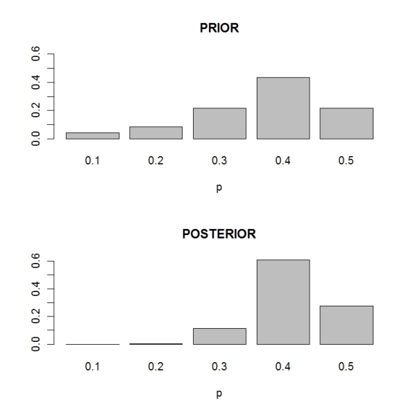Note that the posterior probs are more precise than the prior probabilities.  I am more confident that the proportion of McDonalds fans is equal to 0.4.

Discrete Bayes, part II

In the previous post, I used the R function dexp in my discrete Bayes function.  Sometimes you need to make slight changes to the functions in the R stats package for a given problem.

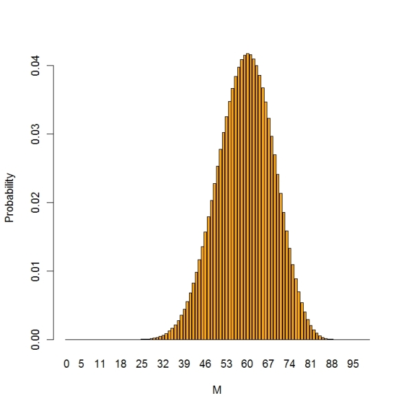
Here is a finite population sampling problem.   A small community has 100 voters and you are interested in learning about the number, say M, who will vote for a school levy.  You take a random sample of size 20 (without replacement) and 12 are in support of the levy.  What have you learned about M?

Here the sampling density is hypergeometric —  the probability that will be in favor out of 20 given that M in the population favor the levy — this is given by the hypergeometric probability

There is a function dhyper that computes this probability, but uses a different parametrization.   So I write a new function dhyper2 that uses my parametrization.

dhyper2=function(x,M,sample.size=n,pop.size=N)

dhyper(x,M,N-M,n)

dhyper2=function(y,M,sample.size=n,pop.size=N)
dhyper(y,M,N-M,n)

Ok, we’re ready to go.  I again read in the special functions to handle the discrete bayes calculations.

source(”http://bayes.bgsu.edu/m6480/R/discrete.bayes.functions.R”)

Here M (the number in favor in the population) can be any value from 0 to 100.  I place a uniform prior on these values.

> prior=rep(1/101,101)

> names(prior)=0:100

I define n (sample size), y (number in favor in sample) and N (population size):

> n=20; y=12; N=100

Now I can apply the function discrete.bayes with inputs dhyper2 (the sampling density), prior, and the observed number in favor.  I indicate also the known sample size and population size.

> s=discrete.bayes(dhyper2,prior,y,sample.size=n,pop.size=100)

By using the plot and summary methods, I plot the posterior for M and display a 90% probability interval.

> plot(s,xlab=”M”,ylab=”Probability”,col=”orange”)

> summary(s)

$coverage

[1] 0.9061118

$set

[1] 44 45 46 47 48 49 50 51 52 53 54 55 56 57 58 59 60 61 62 63 64 65 66 67 68

[26] 69 70 71 72 73 74

We see that P(44 <= M <= 74) = 0.906

Discrete Bayes

One good way of introducing Bayesian inference is by the use of discrete priors. I recently wrote a simple generic R function that does discrete Bayes for arbitrary choice of a prior and sampling density.   I’ll illustrate this function here and in the next posting.

Suppose I’m interested in learning about the rate parameter of an exponential density.  We observe a sample  from the density defined by

where we are interested in learning about the rate parameter .

In R, I read in the function “discrete.bayes” and a few associated methods by typing

> source(“http://bayes.bgsu.edu/m6480/R/discrete.bayes.functions.R&#8221;)

> source(“http://bayes.bgsu.edu/m6480/R/discrete.bayes.functions.R&#8221;)

I define my prior.  I believe the values .05, .10, …, 0.50 are all plausible rate values and I assign each the same prior probability.  In the following R code, prior is a vector of probabilities where I’ve named the probabilities by the values of the rate.

> rate=seq(.05,.50,by=.05)

> prior=rep(.1,10)

> names(prior)=rate

> prior

0.05  0.1 0.15  0.2 0.25  0.3 0.35  0.4 0.45  0.5

0.1  0.1  0.1  0.1  0.1  0.1  0.1  0.1  0.1  0.1

Now I enter in the observations:

> y=c(6.2, 5.0, 1.2, 10.2, 5.9, 2.3, 1.1, 19.0,  4.2, 27.5)

I update my probabilities by the function discrete.bayes — the arguments are the sampling density (dexp), the prior vector, and the data vector.

> s=discrete.bayes(dexp,prior,y)

To display, graph, and summarize these probabilities, I use the generic functions “print”, “plot”, and “summary”.

Here are the posterior probabilities.

> print(s)

0.05          0.1         0.15          0.2         0.25          0.3

2.643537e-02 4.353606e-01 4.037620e-01 1.153126e-01 1.727192e-02 1.719954e-03

0.35          0.4         0.45          0.5

1.292256e-04 7.900085e-06 4.125920e-07 1.903091e-08

To display the probabilities, use “plot”.

> plot(s,xlab=”RATE”,ylab=”PROBABILITY”)

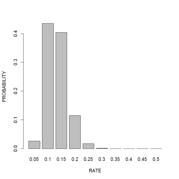To find a 90% probability estimate for the rate, use summary:

> summary(s,coverage=0.90)

$coverage

[1] 0.9544352

$set

[1] 0.10 0.15 0.20

The probability the rate is in the set {0.10, 0.15, 0.20} is 0.95.

Sequential learning by Bayes’ rule

I’m talking about Bayes’ rule now and here’s a quality control example (I think it comes from an intro Bayesian book by Schmitt that was published in the 1960’s):

A machine in a small factory is producing a particular automotive component.

Most of the time (specifically, 90% from historical records), the machine is

2.4 Sequential Learning 7

working well and produces 95% good parts. Some days, the machine doesn’t

work as well (it’s broken) and produces only 70% good parts. A worker inspects

the first dozen parts produced by this machine on a particular morning and

obtains the following results (g represents a good component and b a bad

component):

g, b, g, g, g, g, g, g, g, b, g, b.

The worker is interested in assessing the probability the machine is working

well.

A machine in a small factory is producing a particular automotive component.  Most of the time (specifically, 90% from historical records), the machine is working well and produces 95% good parts. Some days, the machine doesn’t work as well (it’s broken) and produces only 70% good parts. A worker inspects the first dozen parts produced by this machine on a particular morning and obtains the following results (g represents a good component and b a bad component):  g, b, g, g, g, g, g, g, g, b, g, b.  The worker is interested in assessing the probability the machine is working well.

Here we have two models:  W, the machine is working, and B, the machine is broken, and we initially believe P(W) = 0.9 and P(B) = 0.1.  We know the characteristics of each machine.  If the machine is working, it produces 95% good parts, and if the machine is broken, it produces only 70% good parts.

We use the odds form of Bayes’ rule:

Posterior Odds of W = (Prior Odds of W) x BF,

where BF (Bayes factor) is the ratio  P(data | W)/P(data|B).  It is convenient to express this on a log scale:

log Post Odds of W = log Prior Odds of W + log BF

Let’s illustrate how this works.  Initially the prior odds of working is

log Prior Odds = log [P(W)/P(B)] = log(0.9/0.1) = 2.20.

We first observe a good part (g).  The log BF is

log BF = log (P(g | W)/log(g | B)) = log(0.95/0.70) = 0.31,

so the new log odds of working is

log Posterior Odds = 2.20 + 0.31 = 2.51

so we are more confident that the machine is in good condition.

We can continue doing this in a sequential fashion.  Our posterior odds becomes our new prior odds and we update this odds with each observation.  If we observe a good part (g), we’ll add 0.31 to the log odds; if we observe a bad part (b), we’ll add

log [P(b | W) / P(b | B)] = log(0.05/0.30) = -1.79

to the log odds.  I did this for all 12 observations.  Here’s a graph of the results  (first I’ll show the R code I used).

d=c(“g”,”b”,”g”,”g”,”g”,”g”,”g”,”g”,”g”,”b”,”g”,”b”)
log.BF=ifelse(d==”g”,log(.95/.70),log(.05/.30))
prior.log.odds=log(.9/.1)
plot(0:12,c(prior.log.odds,prior.log.odds+cumsum(log.BF)),
type=”l”,lwd=3,col=”red”,xlab=”OBSERVATION”,
ylab=”log odds of working”,main=”Sequential Learning by Bayes’ Rule”)
abline(h=0)

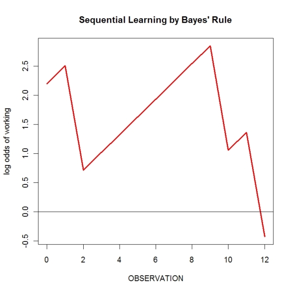After observation, the posterior log odds is -0.43 which translates to a posterior probability of  exp(-0.43)/(1+exp(-0.43)) = 0.39  that the machine is working.  The machine should be fixed.