Sequential Learning in Bayes’ Rule

I have pasted the R code for implementing the quality control example I talked about in class

 

########################################################
# Illustration of function bayes to illustrate
# sequential learning in Bayes’ rule
# Jim Albert, August 2013
########################################################

bayes <- function(prior, likelihood, data){
probs <- matrix(0, length(data) + 1, length(prior))
dimnames(probs)[[1]] <- c(“prior”, data)
dimnames(probs)[[2]] <- names(prior)
probs[1, ] <- prior
for(j in 1:length(data))
probs[j+1, ] <- probs[j, ] * likelihood[, data[j]] /
sum(probs[j, ] * likelihood[, data[j]])
dimnames(probs)[[1]] <-
paste(0:length(data), dimnames(probs)[[1]])
data.frame(probs)
}

# quality control example
# machine is either working or broken with prior probs .9 and .1

prior <- c(working = .9, broken = .1)

# outcomes are good (g) or broken (b)
# likelihood matrix gives probs of each outcome for each model

like.working <- c(g=.95, b=.05)
like.broken <- c(g=.7, b=.3)
likelihood <- rbind(like.working, like.broken)

# sequence of data outcomes

data <- c(“g”, “b”, “g”, “g”, “g”, “g”, “g”, “g”, “g”, “b”, “g”, “b”)

# function bayes will computed the posteriors, one datum at a time
# inputs are the prior vector, likelihood matrix, and vector of data

posterior <- bayes(prior, likelihood, data)
posterior

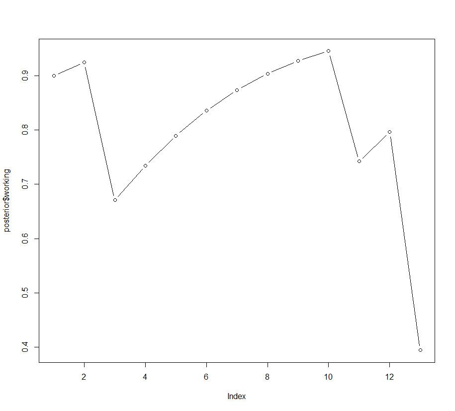
# graph the probs of working as a function of the data observation

plot(posterior$working, type=’b’)

###################################################

Here is the output — the posterior probabilities and the graph.


working broken
0 prior 0.9000000 0.10000000
1 g 0.9243243 0.07567568
2 b 0.6705882 0.32941176
3 g 0.7342373 0.26576271
4 g 0.7894495 0.21055055
5 g 0.8357571 0.16424288
6 g 0.8735119 0.12648812
7 g 0.9035891 0.09641094
8 g 0.9271111 0.07288893
9 g 0.9452420 0.05475796
10 b 0.7420707 0.25792933
11 g 0.7961074 0.20389264
12 b 0.3942173 0.60578268