Bayesian testing of a point null hypothesis

Home > Model checking & comparison > Bayesian testing of a point null hypothesis

Bayesian testing of a point null hypothesis

November 13, 2009 Jim Albert Leave a comment Go to comments

Here is today’s example illustrating a Bayesian test of a point null hypothesis. In Agresti and Franklin’s intro stats book, there is an example wondering if Americans work, on average, 40 hours per week. If $\mu$ represents the mean hours worked per week for all Americans, we are interested in testing $H: \mu = 40$ against the alternative $A: \mu \neq 40$ .

In the example in Agresti and Franklin’s text, a sample of 868 workers were selected and one observes that the workers worked an average of 39.11 hours and one assumes the population standard deviation is equal to $\sigma = 14$ . The test statistic is

$z = \frac{\sqrt{868}(\bar y - 40)}{14} = -1.87$

and one computes a p-value of 0.061. There seems to be moderately significant evidence that the mean working hours for all workers is different from 40.

Here’s an outline of a Bayesian test (I give more details in class):

1. We assign probabilities to the hypotheses $H$ and $A$ . Here we assume each hypothesis is equally likely.

2. Under the hypothesis $H$ , the prior for $\mu$ is a point mass at the hypotheized value of 40.

3. Under the alternative hypothesis, we’ll place a N(40, $\tau$ ) prior on $\mu$ . This reflects the belief that, under the alternative, values of $\mu$ near 40 are more likely that values far from 40.

Under these assumptions, we give (in class) the posterior probability of the hypothesis $H$ . This probability is programmed in the function mnormt.twosided in the LearnBayes package. The inputs to this function are (1) the value to be tested, (2) the prior probability of $H$ , (3) a vector of values of $\tau$ and (4) a data vector consisting of $\bar y, n, \sigma$ . The outputs are the Bayes factor in support of $H$ and the posterior probability of $H$ .

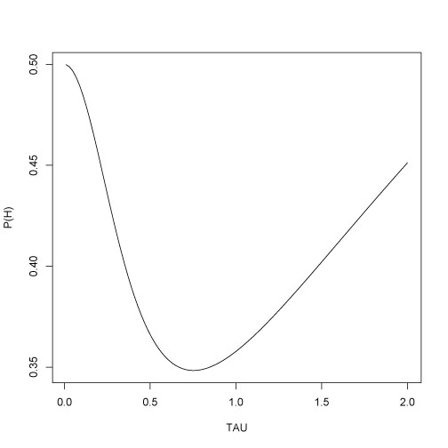
Since it is not clear how to specify the prior standard deviation $\tau$ — we compute the posterior probability for a range of values of $\tau$ . I write a short function to output the posterior probability as a function of $\tau$ and then I use the curve function to plot this probability for values of $\tau$ from 0.01 to 2.

What we see is that the posterior probability of $\mu = 40$ exceeds 0.35 for all values of $\tau$ . This suggests that the p-value overstates the evidence against the null hypothesis.

> data=c(39.11, 868, 14)
> prob.H=function(tau)
+ mnormt.twosided(40,.5,tau,data)$post

Bayesian Thinking