Illustration of posterior predictive checking

To illustrate posterior predictive checking, suppose we observe data y1,…,yn that we assume is N(mu, sigma). We place a noninformative prior on (mu, sigma) and learn about the parameters based on the posterior distribution. We use the posterior predictive distribution to check out model — to see if our sample is consistent with samples predicted from our fitted model.

In practice, we construct a checking function d that is a function of the future sample y*. In this example (66 measurements of the speed of light), we suspect that the smallest observation is an outlier. So we use a checking function d(y) = y_min.

Here’s an R procedure for checking our model using this diagnostic.

We load in the speed of light data:

> y=scan(“speedoflight.txt”)
Read 66 items
> y
[1] 28 22 36 26 28 28 26 24 32 30 27 24 33 21 36 32 31 25 24
[20] 25 28 36 27 32 34 30 25 26 26 25 -44 23 21 30 33 29 27 29
[39] 28 22 26 27 16 31 29 36 32 28 40 19 37 23 32 29 -2 24 25
[58] 27 24 16 29 20 28 27 39 23

We simulate 1000 draws from the normal/scale x inv-chi-square posterior using the function normpostsim.

parameters=normpostsim(y,1000)

The output is a list — here parameters$mu contains draws from mu, and parameters$sigma2 contains draws of sigma2.

The simulation of samples from the posterior predictive distribution is done by the function normpostpred. By use of comments, we explain how this function works.

normpostpred=function(parameters,sample.size,f=min)
{
# the function normalsample simulates a single sample given parameter values mu and sigma2.
# the index j is the index of the simulation number

normalsample=function(j,parameters,sample.size)
rnorm(sample.size,mean=parameters$mu[j],sd=sqrt(parameters$sigma2[j]))

# we use the sapply command to simulate many samples, where the number of samples
# corresponds to the number of parameter simulations

m=length(parameters$mu)
post.pred.samples=sapply(1:m,normalsample,parameters,sample.size)

# on each posterior predictive sample we compute a stat, the default stat is min

stat=apply(post.pred.samples,2,f)

# the function returns all of the posterior predictive samples and a vector of values of the
# checking diagnostic.

return(list(samples=post.pred.samples,stat=stat))
}

Here the size of the original sample is 66. To generate 1000 samples of size 66 from the posterior predictive distribution, and storing the mins of the samples, we type

post.pred=normpostpred(parameters,66)

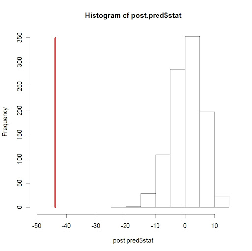
The values of the minimum observation in all samples is stored in the vector post.pred$stat. We display the mins in a histogram and draw a vertical line showing the location of the min of the data.

> hist(post.pred$stat,xlim=c(-50,15))
> lines(min(y)*c(1,1),c(0,350),lwd=3,col=”red”)

Clearly the smallest observation is inconsistent with the mins generated from samples from the posterior predictive distribution. This cast doubts on the normality assumption of the data.